Scale categorical raster map using multi-dimensional grid-point scaling

scales a categorical raster, given a scaling factor and user-defined label precision

mdgp_scale_raster(
  raster,
  class_field,
  scale_factor,
  parts,
  rpr_threshold,
  monotypic_threshold
)

Arguments

raster

categorical spatial raster (terra SpatRaster) with class names in an attribute field

class_field

attribute field in the SpatRaster that contains the class names

scale_factor

ratio of lower (scaled) resolution to higher (original) raster resolution (resolution of lower resolution divided by resolution of higher resolution)

parts

integer - precision of class labels in parts (1 = 100%, 2 = 50%, 3 = 33.3%, 4 = 25%, 5 = 20%)

rpr_threshold

integer - minimum percentage of grid cell in scaled landscape to be represented by a class

monotypic_threshold

integer - minimum percentage of fine resolution class in a scaled grid cell grid to be considered monotypic

Value

List with 3 objects. Two SpatRaster objects and a list with two objects.

The two scaled raster results are a categorical SpatRaster object with the scaled classified map and scaled class labels in the attribute table, and a numeric SpatRaster object with cell-level information retention. The second object contains a data frame with class-specific information retention and landscape-scale information retention.

See also

relative_abundance_scaled_grid to generate relative abundance for each scaled grid cell, mdgp_scale classifying relative abundance samples to multi-dimensional grid points, and scaling_result_to_raster converting scaling result to spatial raster and info_retention_stats.

Examples

# load categorical raster
r <- terra::rast(system.file("extdata/nlm_mid_geom_r3_sa0.tif", package = "landscapeScaling"))

# subset the raster to the lower 300 by 300pixels
r_sub <- terra::crop(r,terra::ext(0,300,0,300))

# scale the original map with class name field 'cover'
# scaling parameters: scale factor = 15, parts = 3, 
# representativeness threshold = 10%, and monotypic threshold = 90%
scaled_map <- mdgp_scale_raster(r_sub,'cover',15,3,10,90)
#> [1] "number of cells: 400"
#> [1] "number of grid points: 10"
#> [1] "number of grid points remaining: 5"

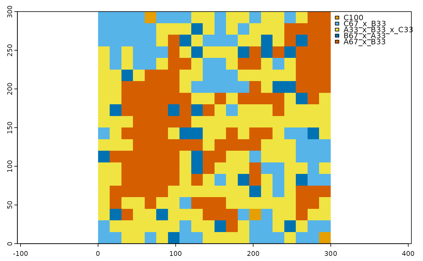
# plot the scaled raster
# scaled color scheme for six lasses
clr_scale <- c('#E69F00','#56B4E9','#009E73','#F0E442','#0072B2','#D55E00')
terra::plot(scaled_map[[1]],col=clr_scale,mar=c(1.5,1.5,1,1))


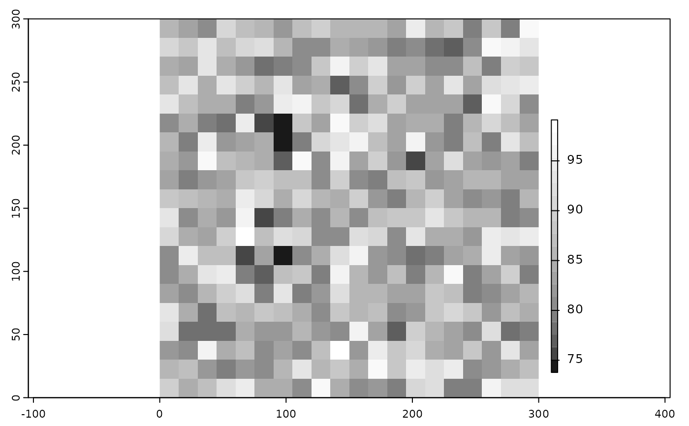
# plot the information retention raster
terra::plot(scaled_map[[2]],plg=list(ext=c(310,315,20,220),loc = "right"),
col=gray.colors(20,start=0.1,end=1),mar=c(1.5,1.5,1,1))