Convert scaling result to spatial raster
Source:R/scaling_result_to_raster.R
scaling_result_to_raster.Rdconverts the scaling result of mdgp_scale() to spatial raster objects#'
scaling_result_to_raster(
  scaling_result,
  class_name_field,
  proj_info = NA,
  scale_factor
)
Arguments
- scaling_result
data frame with scaling results generated by function mdgp_scale
- class_name_field
field name that contains scaled class names
- proj_info
projection information of coordinates in the data frame to be converted to raster
- scale_factor
ratio of lower (scaled) resolution to higher (original) raster resolution (resolution of lower resolution divided by resolution of higher resolution)
Value
List with 3 objects. Two SpatRaster objects and a list with two objects.
The two scaled raster results are a categorical SpatRaster object with the scaled classified map and scaled class labels in the attribute table, and a numeric SpatRaster object with cell-level information retention. The second object contains a data frame with class-specific information retention and landscape-scale information retention.
See also
relative_abundance_scaled_grid to generate relative abundance for each scaled grid cell,
mdgp_scale classifying relative abundance samples to multi-dimensional grid points.
Examples
# load categorical raster
r <- terra::rast(system.file("extdata/nlm_mid_geom_r3_sa0.tif", package = "landscapeScaling"))
# subset the raster to the lower 300 by 300 pixels
r_sub <- terra::crop(r,terra::ext(0,300,0,300))
# generate relative abundance for the scaled grid
rel_abund <- relative_abundance_scaled_grid(r_sub,class_field='cover',scale_factor=15)
head(rel_abund)
#> x y A B C
#> 1 0 0 4.8888889 38.22222 56.88889
#> 2 15 0 10.2222222 38.66667 51.11111
#> 3 30 0 20.0000000 42.66667 37.33333
#> 4 45 0 24.8888889 40.44444 34.66667
#> 5 60 0 0.8888889 28.00000 71.11111
#> 6 75 0 17.7777778 37.33333 44.88889
# classify relative abundance samples to multidimensional grid points
mdgp_result <- mdgp_scale(rel_abund,parts=3,rpr_threshold=10,monotypic_threshold=90)
#> [1] "number of cells: 400"
#> [1] "number of grid points: 10"
#> [1] "number of grid points remaining: 5"
head(mdgp_result)
#> cls A B C x_y prc_inf_agr class_name
#> 1 10 0.000 8.444 91.556 285_0 91.556 C100
#> 2 10 0.000 9.333 90.667 195_30 90.667 C100
#> 3 10 0.444 12.444 87.111 60_285 87.111 C100
#> 4 9 4.889 38.222 56.889 0_0 90.222 C67_x_B33
#> 5 9 10.222 38.667 51.111 15_0 84.444 C67_x_B33
#> 6 9 10.667 42.667 46.667 225_0 80.000 C67_x_B33
# rasterize the scaling result
scaled_map <- scaling_result_to_raster(mdgp_result,class_name_field='class_name',scale_factor=15)
print(scaled_map)
#> [[1]]
#> class : SpatRaster
#> dimensions : 20, 20, 1 (nrow, ncol, nlyr)
#> resolution : 15, 15 (x, y)
#> extent : 0, 300, 0, 300 (xmin, xmax, ymin, ymax)
#> coord. ref. :
#> source : memory
#> categories : class_name
#> name : class_name
#> min value : C100
#> max value : A67_x_B33
#>
#> [[2]]
#> class : SpatRaster
#> dimensions : 20, 20, 1 (nrow, ncol, nlyr)
#> resolution : 15, 15 (x, y)
#> extent : 0, 300, 0, 300 (xmin, xmax, ymin, ymax)
#> coord. ref. :
#> source : memory
#> name : prc_inf_agr
#> min value : 73.778
#> max value : 99.111
#>
#> [[3]]
#> [[3]][[1]]
#> class_name freq class_id prop inf_retention_mn inf_retention_sd
#> 1 A33_x_B33_x_C33 165 1 0.4125 84.129 3.814
#> 2 A67_x_B33 122 2 0.3050 87.417 6.519
#> 3 B67_x_A33 29 3 0.0725 82.038 2.214
#> 4 C100 3 4 0.0075 89.778 2.352
#> 5 C67_x_B33 81 5 0.2025 88.093 5.132
#>
#> [[3]][[2]]
#> mean sd
#> information_retention_landscape 85.826 5.356
#>
#>
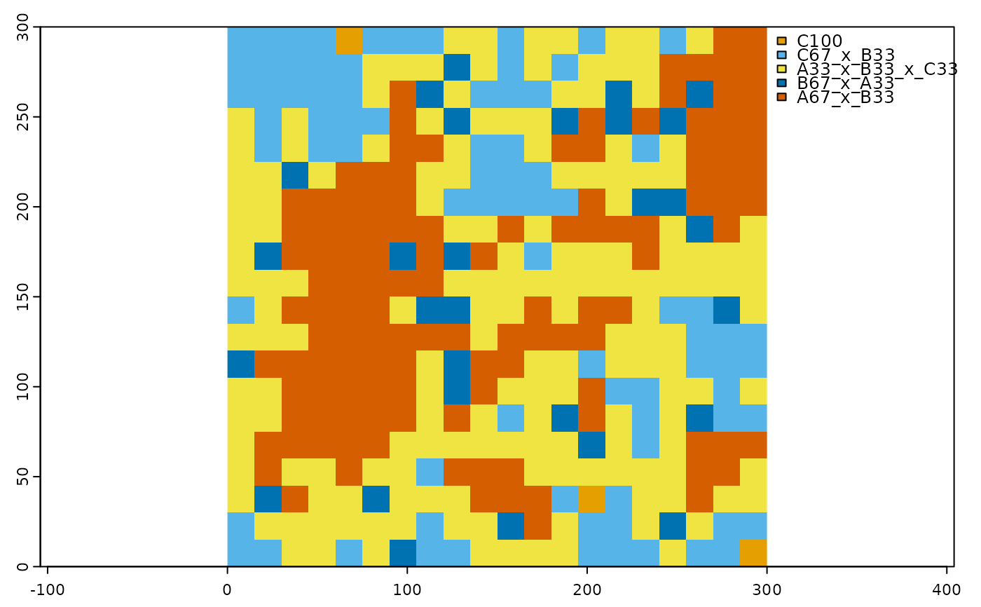
# plot the scaled raster
# scaled color scheme for six lasses
clr_scale <- c('#E69F00','#56B4E9','#009E73','#F0E442','#0072B2','#D55E00')
terra::plot(scaled_map[[1]],col=clr_scale,mar=c(1.5,1.5,1,1))
 # plot the information retention raster
terra::plot(scaled_map[[2]],plg=list(ext=c(310,315,20,220),loc = "right"),
col=gray.colors(20,start=0.1,end=1),mar=c(1.5,1.5,1,1))
# plot the information retention raster
terra::plot(scaled_map[[2]],plg=list(ext=c(310,315,20,220),loc = "right"),
col=gray.colors(20,start=0.1,end=1),mar=c(1.5,1.5,1,1))
