landscapeScaling
landscapeScaling
![]()
The purpose of the “landscapeScaling” package is to provide methods and functions to upscale categorical raster data. The recommended method is the multi-dimensional grid-point (mdgp) scaling algorithm. It generates a new classification scheme on the basis of user desired class label precision of mixed classes and representativeness of the scaled class across the landscape of interest. The scaling output includes scaled categorical raster maps with mixed classes, a corresponding continuous raster with information retention calculations for each scaled grid cell and class-specific and landscape-scale information retention mean and standard deviation. The alternative method available in the package that does not modify the classification scheme is the majority (plurality) rule.
Installation
You can install the development version of landscapeScaling from GitHub with:
# install.packages("devtools")
devtools::install_github("gannd/landscapeScaling")
library(landscapeScaling)
library(terra)
#> terra 1.8.54
Example
For demonstration purpose we will load a package provided landscape with three classes and first subset the original raster to the lower left chunk of 660 by 660 grid cells.
# three class color scheme
clr <- c('#332288','#44AA99','#DDCC77')

# scaled color scheme
clr_scale <- c('#56B4E9','#009E73','#F0E442','#0072B2','#D55E00','#000000')

# load categorical raster data set and plot
r <- terra::rast(system.file("extdata/nlm_mid_geom_r3_sa0.tif", package = "landscapeScaling"))
terra::plot(r, col=clr,mar=c(1.5,1.5,0.75,5))

# generate subset extent to the lower left 660 by 660 cells (demo purpose) and add to plot
sub_ext <- terra::ext(0,660,0,660)
terra::plot(sub_ext, border='white',lwd=2,add=TRUE)
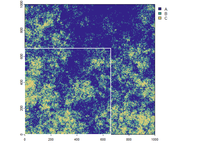
The original raster with three classes and the subset extent in the lower left corner (outline in white).
# subset the landscape and plot
r_sub <- terra::crop(r,sub_ext)
terra::plot(r_sub,col=clr,mar=c(1.5,1.5,0.75,5))
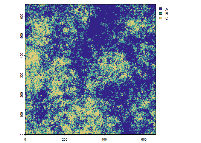
The subset of the categorical raster.
Scaling Process Steps
1) Generate the scaled grid with the “scale_grid” function applying a scale factor of 15. First the lower left corner of the 15 by 15 grid cells will be generated.
# generate the scaled grid
LL_pnts <- scale_grid(r_sub,scale_factor=15)

# print the first 10 rows of the generated coordinates
head(LL_pnts,10)
#>      x y
#> 1    0 0
#> 2   15 0
#> 3   30 0
#> 4   45 0
#> 5   60 0
#> 6   75 0
#> 7   90 0
#> 8  105 0
#> 9  120 0
#> 10 135 0

# plot the subset raster and overlay hte scaled grid cell outline
terra::plot(r_sub,col=clr,mar=c(1.5,1.5,0.75,5))
terra::plot(vect(LL_pnts,geom=c("x","y")),pch=3,col='#EEEEEE',add=TRUE)
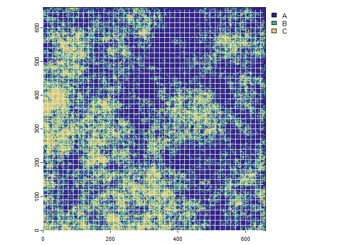
The subset of the categorical raster and the scaled grid cell origin (lower left corners)
2) Generate relative abundance for the subset for a scale factor of 15. First the lower left corner of the 15 by 15 grid cells will be generated. The relative abundance for each of the 44 x 44 scaled grid cells and the relative abundances are returned as a data frame.
# generate relative abundance
rel_abund <- relative_abundance_scaled_grid(r_sub,class_field='cover',scale_factor=15)

# print the first 10 rows of the resulting data frame
head(rel_abund,10)
#>      x y          A        B        C
#> 1    0 0  4.8888889 38.22222 56.88889
#> 2   15 0 10.2222222 38.66667 51.11111
#> 3   30 0 20.0000000 42.66667 37.33333
#> 4   45 0 24.8888889 40.44444 34.66667
#> 5   60 0  0.8888889 28.00000 71.11111
#> 6   75 0 17.7777778 37.33333 44.88889
#> 7   90 0 25.7777778 58.22222 16.00000
#> 8  105 0  9.3333333 42.66667 48.00000
#> 9  120 0  0.8888889 35.11111 64.00000
#> 10 135 0 22.2222222 49.33333 28.44444
3) Classify the relative abundance of each scaled grid cell to a list of multi-dimensional grid points. First the multi-dimensional grid points are generated, then each grid cell is classified to the grid point that maximizes information retention. Grid points are generated from the class label precision parameter $parts$ and the landscape richness (number of classes). The mdgp_scale function requires the argument $parts$ for the class label precision, the representativeness threshold ($prp-threshold$), the monotypic class threshold ($monotypic-threshold$), and the cell-level information retention threshold ($ir-threshold$). The information retention threshold reclassifies cells with information retention less than the threshold to a class “OTHER”. This class is actually called “ZZZ_OTHER” to ensure that the “OTHER” class is added at the end of the scaled class list.
In this example we will a 33.3% class label precision, a 10% representativeness threshold, a 90% monotypic class threshold, and a cell-level information retention threshold of 75%.
# classify relative abundance samples to multidimensional grid points
mdgp_result <- mdgp_scale(rel_abund,parts=3,rpr_threshold=10,monotypic_threshold=90,ir_threshold=75)
#> [1] "number of cells: 1936"
#> [1] "number of grid points: 10"
#> [1] "number of grid points remaining: 6"
#> [1] "number of grid points remaining: 5"

# list the first 10 records of the mdgp scaling result
head(mdgp_result,10)
#>    cls     A      B      C     x_y prc_inf_agr class_name
#> 1   10 0.000  8.444 91.556   285_0      91.556       C100
#> 2   10 2.222 10.667 87.111  15_390      87.111       C100
#> 3   10 0.000 12.889 87.111  30_390      87.111       C100
#> 4   10 0.000  9.333 90.667  195_30      90.667       C100
#> 5   10 0.000  5.778 94.222  45_390      94.222       C100
#> 6   10 0.000  5.333 94.667  15_360      94.667       C100
#> 7   10 0.000 12.889 87.111 315_105      87.111       C100
#> 8   10 0.444  3.111 96.444  30_405      96.444       C100
#> 9   10 0.000  4.000 96.000   0_360      96.000       C100
#> 10  10 0.444  8.444 91.111  45_375      91.111       C100

# tabulate the final class frequencies
table(mdgp_result$class_name)
#>
#>            A100 A33_x_B33_x_C33       A67_x_B33            C100       C67_x_B33
#>             330             652             735              12             204
#>       ZZZ_OTHER
#>               3
Notice the “ZZZ_OTHER” class with the highest class value.
4) Convert classified points to raster and location-specific information retention and summarize information retention at the class-level and across the scaled landscape with the function scaling_result_to_raster().
# convert classified points and location-specific information retention to raster
mdgp_raster <- scaling_result_to_raster(mdgp_result,class_name_field='class_name',scale_factor=15)

# show the class levels of the scaled categorical raster data
levels(mdgp_raster)
#> NULL

# plot the scaled map
terra::plot(mdgp_raster[[1]],col=clr_scale,mar=c(1.5,1.5,1,8))
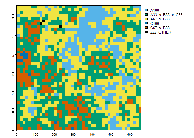
The scaled categorical raster with the scaled classification scheme.
# plot information retention of the scaled map
terra::plot(mdgp_raster[[2]],col=gray.colors(20,start=0.1,end=1),mar=c(1.5,1,1,8))
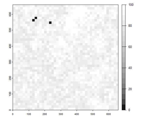
Information retention raster at the scaled grid cell level. Note that the information retention for the “ZZZ_OTHER” class is set to 0.
The class-specific and landscape-level information retention mean and standard deviaitons can be retrieved from the third object returned by the function scaling_result_to_raster().
# print the class-specific and landscape scale summary statistics
print(mdgp_raster[[3]])
#> [[1]]
#>        class_name freq class_id        prop inf_retention_mn inf_retention_sd
#> 1            A100  330        1 0.170454545           92.174            5.085
#> 2 A33_x_B33_x_C33  652        2 0.336776860           83.679            4.130
#> 3       A67_x_B33  735        3 0.379648760           89.385            5.293
#> 4            C100   12        4 0.006198347           91.667            3.917
#> 5       C67_x_B33  204        5 0.105371901           87.954            5.226
#> 6       ZZZ_OTHER    3        6 0.001549587            0.000            0.000
#>
#> [[2]]
#>                                   mean    sd
#> information_retention_landscape 87.663 6.759